RS/AS AND NUGGET ZONE SEM ANALYSIS AND MATHEMATICAL EQUATIONS FOR PARAMETER OPTIMIZATION ON FRICTION STIR WELDING TOOL
Yugandhar Meka 1; Prabhakar Kammar 2
1 Department of Mechanical Engineering, Research scholar, (New Horizon College of Engineering, Benga-luru), Bengaluru, India-560103
2 Department of Mechanical Engineering, Professor, (Gopalan College of Engineering and Management), Bengaluru, India-560048b>
e-mail: yugandhar077@gmail.com Phone: +91 6301012889.
ABSTRACT
In order to find the ideal process parameters, the friction stir welding (FSW) production process is combined with mathematical optimisation techniques in the current thesis. In terms of optimisation, the goals (or objec-tives) are process- related in that they define or represent how the process behaves. The Welding Institute (TWI),UK introduced the FSW process, which has been enhanced in this study, as a relatively new welding tech-nology in 1991. In conclusion, because the process is solid-state and does not involve melting, many of the problems of conventional fusing welding techniques may be avoided. In the FSW process, two work pieces are submerged in a spinning tool. As a result of friction and plastic dissipation, the temperature rises to the point where the material is sufficiently softened to be mixed together, forming a weld.Involving solid material ow, heat transmission, thermal softening, recrystallization, and the production of residual stresses, the process is mul-tiphysics in nature.
Keywrods: magnesium alloys, friction stir welding tensile strength, tensile elastic limit, Young’s modulus, Poisson’s ratio, yield strength, strain-hardening characteristics, AZ91.
Recibido: 03 de septiembre de 2023Aceptado: 20 de diciembre de 2023
Received: September 03, 2023Accepted: Accepted: December 20, 2023

Cómo citar este artículo: M.Yugandhar, Prabhakarkamma. RS/AS and nugget zone SEM analysis and mathematical equations for parameter optimization on friction stir welding tool”, Revista Politécnica, vol.20, no.39 pp.78-98, 2024. DOI:10.33571/rpolitec.v20n39a6
1. INTRODUCTION
The purpose of this work is to use numerical modeling and optimization tools to study and control thermo-mechanical conditions, ie residual stresses and workload conditions, in friction stir welding (FSW) process-es. Since the 1990s, various theoretical/experimental studies and EU-funded industry initiatives such as JOIN-DMC and DEEPWELD have been conducted to better understand the many physical components of the FSW process. rice field. FSW is already used in regular and critical applications for joining structural components, mainly made of aluminum and its alloys. However, further research is still being done to achieve a more robust "process window".
FSW modeling includes a wide range of models such as microstructural evolution, material flow, heat flow, heat generation, residual stress, mechanical loads (such as tool forces) and bond strength. To gain a deep-er understanding of some of the basic mechanisms of the FSW process, the physics is divided into sub-systems, namely thermal and mechanical behavior, and then integrated modeling approaches (1–5 ) is being performed. Compare these two physical aspects with the actual load cases. Microstructural evolution, mate-rial flow, heat flow, heat generation, residual stresses, mechanical loads (such as tool forces), and bond strength are all part of FSW modeling. In order to better understand some of the underlying mechanisms of the FSW process, we divided the physics into subsystems, namely thermal and mechanical behavior, and used an integrated modeling approach to study these two physical aspects. combined the combined be-havior of the with the actual behavior. load case.
Most of the work done in the current research study has been devoted to computer models of various components of the FSW process (6). In particular, heat diffusion and transient/residual stresses occurring during and after welding were investigated numerically and compared with published experimental data. Therefore, important information on the development of residual stresses as a function of key FSW pro-cess parameters such as tool rotation speed and cross-welding speed was collected using the general-purpose Nite Elements (FE) software ANSYS (Ansys Inc., 2007). will be, ABAQUS (Dassault Systèmes, 2007) and COMSOL (COMSOL AB, 2007) [8].
Following our modeling studies, we used numerical optimization techniques, including classical and evolu-tionary algorithms, to find the optimal process parameters.
2. EXPERIMENTAL WORK
FSW is a tool with a threaded/unthreaded cylindrical/probe shoulder [9]. As shown in Figure 1.1, the probe (pin) rotates at a constant speed and travels at a constant travel speed in the connecting line between the two butt- welded sheets or plates of material. The part must be firmly secured to the backing plate to sup-port the high plunge pressure of the FSW machine head (7) and prevent the adjacent mating surfaces from being pushed apart. The pin length should be slightly less than the desired weld depth and the tool shoulder should be in direct contact with the workpiece surface. Insert the probe into the workpiece and move the tool along the weld at a 2-4 degree bevel angle to increase pressure under the tool shoulder.
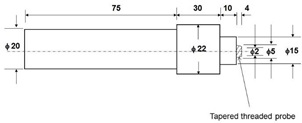
Fig .1. A schematic diagram of taper tool

Fig .2. A diagram of the FSW process
Frictional heat is generated between the wear- resistant welding tool shoulder [10] and the pin, and on the other hand with the work material. This heat, combined with the heat generated by plastic dissipation during the mix-ing process, softens the agitated components without reaching their melting point (hence the name solid-state process), leaving the tool in a plasticized tubular shape. Allows crossing metal weld lines. When the pin is pushed in the welding direction, the front of the pin pushes the plasticized material into the back of the pin, applying a large forging force to strengthen the weld metal [11].
Welding of materials is facilitated by strong plastic deformation in the solid state accompanied by dynamic re-crystallization of the weld nugget.
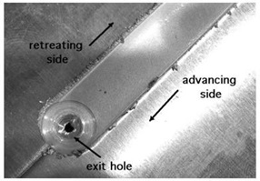
Figure.3.(a) Frictiction stir welding on magnesium sheets
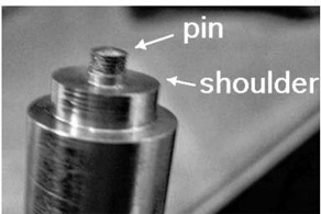
Figure 3.(b) H13 tool steel tool pin and shoulder
The solid-state nature of the FSW process, along with its specific tooling and asymmetric nature, results in a very unique microstructure [12]. Certain areas are common to all weld types, while others are unique to her FSW process. Nomenclature varies, but the following reflects general consensus.
The stirring zone (also called nugget or dynamic recrystallization zone) D in Figure 1.3 is a highly deformed re-gion of material that roughly corresponds to the position of the pin during welding [13]. Particles in the stir zone are nearly equiaxed and are often ten times smaller than those of the starting material (Murr et al., 1997). The extensive presence of many concentric rings in the stirring zone is called the onion ring structure. The spe-cific origin of these rings has not yet been determined, but differences in particle number density, grain size, and organization have been suggested [14].
The flow arm is at the top of the weld and consists of material that is pulled by a shoulder from the retracting side of the weld behind the tool and deposited on the advancing side of the weld [15].
The thermo-mechanically affected zone (TMAZ), represented by the letter C in the figure. 1.3, located on both sides of the stirring zone. The stresses and temperatures in this region are lower than in the stir zone, so the microstructural impact of welding is also less. In contrast to the stir zone, the microstructure is clearly recog-nizable as that of the starting material, albeit clearly distorted and rotated. Although the term TMAZ theoretically refers to the entire deformation area, it is commonly used for areas not yet covered by the terms 'touch zone' and 'forearm' [16].
A heat affected zone (HAZ), represented by B in Figure 1.3, exists in all welding processes.
As the name suggests, this zone is subject to thermal cycling but does not deform during welding. Although the temperature is lower than TMAZ, it can be affected if the microstructure is thermally unstable. In fact, this range is often the lowest mechanical property for heat treatable aluminum alloys [17].
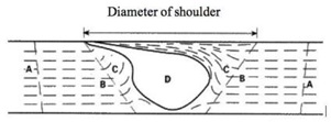
Fig.4. A diagram of the weld zone with several areas..

Figure .5: friction stir welding AZ-31B

Figure 6: Various tool pin geometries used for making joints.
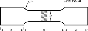
Figure 7: Dimensions of tensile specimen[18]
Table 1: Chemistry of ZE-41 Mg alloy used
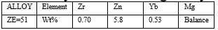
Table 2: Mechanical behavior of parent material ZE-51.
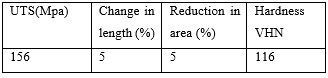
Table 3: Process parameters used
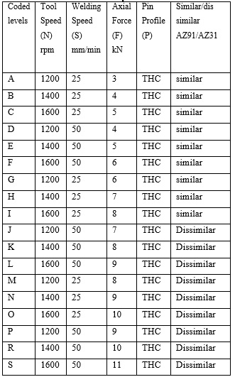
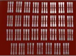
Figure 8: Specimens for tensile testing.
Table 4: ANOVA for developed model [21].
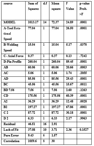
Table 5: Results from ANOVA test for UTS [22]


Figure 9(a) Material clamping_specimen

Figure 9(b) Material holding under 2 jaws
3. THERMAL MODELING OF FSW
3.1. Governing Equations
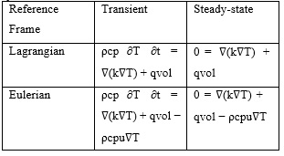
All thermal models, regardless of their complexity, are based on solving the classical heat equation (equation 1). (2) is known in mathematics as a scalar partial differential equation (PDE) (Betounes, 1998; Carslaw and Yeter, 1959). With proper initial and boundary conditions, this time-dependent problem can be solved with both Lagrangian and Eulerian reference systems. In the first scenario the heat field is defined by a fixed coordinate system, whereas in the second scenario the coordinate system moves with the heat source, as shown schemat-ically in Figure 2. In the Lagrangian frame of reference, the temperature change of a region over time is ex-pressed as [23]:

where the constant component K/ρcp , is the material's thermal diusivity, which is a measure of how quickly heat is transferred in a solid.
ρ denotes the material density=kg/ m3
cp the specific heat capacity =J/kg K
T the temperature field (K)
k the thermal conductivity=W/mK
qvol the volumetric heat source term =w/ m3

A convective term is introduced to Eq. when describing heat flow in an Eulerian reference frame (2).

where u is the velocity eld vector, which can include both the tool welding velocity and the material ow eld sur-rounding the tool probe, i.e. in the shear layer.
If transitory effects are insignificant, the time- dependent component, i.e. T t, disappears, and Eq. (2.1) in the Lagrangian reference frame is simplified to
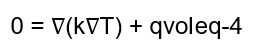
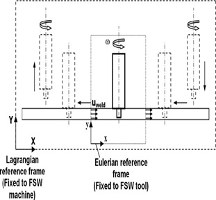
Fig.10.A diagram of the Lagrangian and Eulerian reference frames

The former strategy is relatively common, while the latter can benefit from the steady-state conditions that can occur with moving heat sources [24]. Table 2.1 provides a tabular overview of these formulations. In addition to specific numerical applications, it also provides important analytical formulas. This is discussed in detail in the next section [21]. The combination of frame of reference and interdependence of modeling layers provides a wide range of choices, and the 'right' decision depends on the purpose of the particular model. For example, residual stress models require temperature fields from transient Lagrangian thermal models [25].
Table-6.governing (heat conduction) equations in thermal models in many reference frames and temporal domains.
3.2. Application of the Thin-Plate Solution in FSW
Equation 1 shows a schematic diagram of a linear heat source moving with constant velocity along a line in an infinite plate. The same partial differential equation of heat conduction, including the convec-tive coefficient, governs the temperature field, as shown in Equation 3. Under the quasi-steady state as-sumption given by Eq., the closed solution is given by Eq.-6 [28].
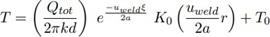
where (Qtot/d) defines the heat input per unit thickness, ξ denotes the moving coordinate axis
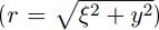
a is the heat diffusivity, K0 denotes the Modified Bessel Function of the second kind and zeroth order and T0 defines the ambient temperature [33].

Fig.11(a) Schematic view of a line-type heat source moving along the joint line of the work piece[26]
shows the resulting temperature profile along the weld axis at various distances, i.e., y = 0, 5, 10, 15 and 20 cm from the bond line, when the heat source passes x = 0 m. increase. Note the infinite temperature mathemat-ical singularity at the heat source location. This is not possible in his real FSW application where the solidus temperature is the limit of the peak temperature [27].
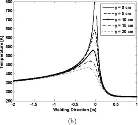
Fig.11(b) Temperature profile along x-axis at different y- points
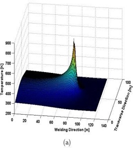
Fig.12. (a) Temperature weld on a 3 mm-thick plate
3.3. Prescribed heat source models in FSW.
Heat generation due to a combination of friction and plastic dissipation is often simulated in most purely thermal FSW models using a surface Ux boundary condition at tool/matrix contact [33]. The most important unknowns in these surface Ux equations are either the friction coefficient under the slip assumption or the material yield stress under the stick assumption [30].
Along this line, Schmidt and Hattel (2004) have proposed the following generally adopted equation for the total heat generation [W],

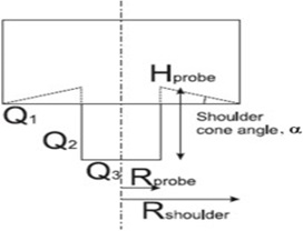
Fig-13. Schematic view of analytical tool geometry (including conical shoulder and cylindrical probe and heat generation contributions from shoulder Q1, probe side Q2 and probe tip Q3).
However, when implementing this into a numerical model using a position dependent surface flux [W/m2 ], it is typically used on the following form[31].

Equation 9
It is the foundation for the equation, Eq (7). Furthermore, by combining Eqs. (7) and (8) and assuming the simple tool shape of an at shoulder, the following well-known formula for heat generation is obtained [32].
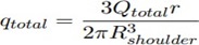
Equation-10
It can be used as a radius-dependent surface UX for models assuming continuous contact or stick states close to sliding when the 14 shear layers are very thin [34].
Qtotal can be viewed as an input parameter in the same way as friction coefficient, pressure, and material yield stress in equation (1). (9). & (7). Note, however, that one of the model's input parameters, Qtotal, can some-times conflict with the underlying goals of FSW thermal modeling. This is especially true if the model is to es-timate temperature in situations not supported by measurements of the total heat input Qtotal [35].
In such cases, the total heat release Qtotal is a function of these parameter variations and can be considered an internal function of the FSW process, making it difficult to predict or simulate the effects of welding or rotational speed variations. This is in contrast to other welding processes such as TIG where the heat input is controlled externally [36].

Fig-14. The left-hand column represents the sliding condition, and the right-hand column represents the stick-ing state; the first row depicts no probe heat production, the second row depicts probe heat generation, and the third row depicts probe volume eliminated and heat generation in the shear layer [34].
4. DISCUSIÓN
4.1. Steady-state Eulerian models with prescribed heat source.
Modeling the whole welding process, including plunge, dwell, and pull out times, entails some significant complications. To lower the computational cost of the moving heat source while maintaining applicability, just the welding time is considered, and a moving coordinate system placed on the heat source is used [35,38].
Eq. (2.2) generalizes heat transport in the plate and is modified into Eq. (2.5) as discussed in Section 2.1.1. The tool's traverse motion is represented by a material ow through the rectangular plate area. The equation in-cludes a convective term in addition to the conductive term due to the ow prescription [36].
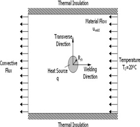
Fig.15.Schematic view of the numerical model with boundary conditions.
where Qtot signifies the total heat input, d the thickness of the shear layer under consideration, and r the ra-dius originating at the tool's center [37].

Figure .16: Schematic view of tool geometry with applied linear heat source on tool shoulder in 2D thermal model.
The modeling includes magnesium parameters for the work material of a plate with a thickness of 3 mm. The welding speed is 2 millimeters per second. The maximum temperature is about 800 K, caused by tem-peratures above the ideal average temperature of 500 °C on the shoulder region. This is physically implau-sible as the solidus temperature Tsol was chosen to be 500 ¿°C (' 773 K) in this scenario. However, this is due to the use of the basic heat source model [40].
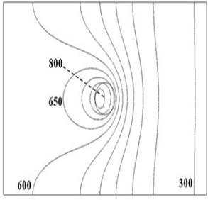
Figure 17: Contour plot of the temperature field. Increment between isotherms is 50 K [38].
Case-1a considers the full sliding contact situation at the tool shoulder/matrix interface, in which the contact shear stress (contact = friction= P) is smaller than the material yield shear stress, resulting in no workpiece de-formation [39].
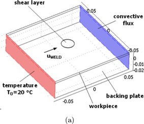
Fig.18.(a) Geometry of the 3D Eulerian thermal model with boundary conditions

Fig.18.(b) Closer view of the shear layer and prescribed velocity field.
Figures 10 and 11 show cylindrical volumes representing shear layers. As already explained in section Equation-3, the surface heat flux acts as a boundary condition for the steady-state heat transfer equation [41], Equation 3. (Five). Case 1b considers the condition of perfect adhesive contact at the tool shoulder-matrix interface. In this case, the friction shear stress is greater than the matrix flow shear stress, indicating that the matrix is deforming at the same speed as the tool rotation speed (1 rotation). segment). The top of the die sticks to the surface of the tool). A strained layer is formed because the ground matrix is stationary against the shoulder matrix contact [1-15].
As shown. You can see the effect of this layer in Figure 9 using a ramp factor that vertically scales the velocity of the segments in the volume. In this scenario the heat source is applied as a volumetric heat flow (qvol in the equation) in a thin shear layer (5). Figure 10 shows the thermal field obtained for case 1b, and Figure 11 shows the asymmetric temperature distribution around the shear layer [8-12].

Figure .19. (a) Temperature field
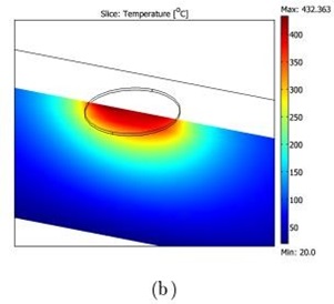
Fig.19.(b) A cross-sectional view of the temperature field around the shear layer, notice the asymmetric temperature distribution due to the material flow in the shear layer[8,9,10,12,14].
The variation in temperature distribution between examples 1a and 1b is visible in the thermal difficulties shown in Figures 11 and 12. It is roughly 15 °C at a distance from the centre equal to half the tool shoulder radius, as visible, notably on the retreating side [15-25].

Fig.20.(a) Comparison of the thermal profiles along the transverse direction through the center of the heat source at the top surface

Fig.20.b. (b) Closer view of the thermal proles in the diameter of the tool shoulder.
Use this diagram to analyze specimen failure at the center of the tool. H. Examine where the weld is formed to determine the length of strain [21,25,27] and the stress/Sterling ratio under the weld. This graph, based on Figure (6-22), yielded the following values:
Tensile strength:69.12MPa, yield point:
60.12 MPa and elongation:1.14 percent. Following this test, micro-Vicker hardness is described using samples from the previous micro-test. Figure 7 shows the effect of welding speed on UTS.
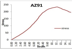
Fig.21. Stress-Strain images for AZ91
We found the minimum welding speed for UTS. UTS increased with increasing welding speed, reached a maximum value, and then decreased with increasing welding speed. The same trend was observed for dif-ferent tool geometries. According to Emam and Domiaty [27], lower welding speeds lead to higher heat input per unit weld length. As the heat input increases, the temperature of the agitation zone rises and the agitation zone cools slowly, forming coarse grains and lowering the UTS.
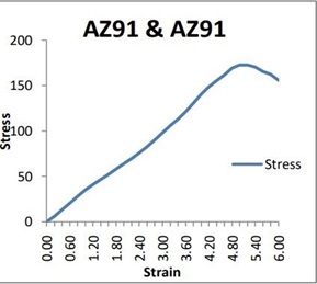
Fig.22.Stress-Strain images for AZ91/AZ91.
In addition, particles with multiple lower bounds indicate poor joints at low welding speeds. This results in lower UTS for joints with welding speeds less than 10 mm/min. Increased welding speed improves the fric-tion effect between workpiece and tool. Heat generation in the weld zone increases with increasing tool- workpiece contact [28].
Figure 7 shows the effect of welding speed on UTS. The lowest UTS welding speed has been found. UTS increased with increasing welding speed, reached a peak, and then began to decline. The same trend was observed for all tool geometries.
According to Emam and Domiaty [27], lower welding speeds lead to higher heat input per unit weld length. Increased heat input increases the temperature of the agitation zone, slowing the cooling process and lead-ing to the formation of coarse particles that cause UTS degradation. In addition, particles with multiple lower bounds and low perspiration rates indicate weak binding. For this reason, joints with a slow welding speed of 10mm/min will have a lower UTS. As the welding speed increases, the frictional motion between the tool and workpiece increases. As the tool-workpiece contact increases, so does the heat dis-sipation in the weld zone [28].
Researchers define models in model specifications by identifying each model. 2 Identify the model. All model parameters have a single solution for a particular model. Estimate the model in step 3. The specified model con-tains parameters whose values should be estimated using sample data.

Fig.23. Nugget Zone Material composition at SEM Analysis
Figure 6 (a, b, c) show SEM images of the crack surface of the tensile specimen. Cracks were formed in the heat affected zone of the FSw bonding process. Macrophotographs show small and brittle surface morpholo-gies of the milled surface. Macrocharts also show sharp drops that may indicate casting defects [34,36].
surface. The magnification of Sem is 80x. Figure 6.3 shows a view of the fracture surface at 100x magnification [12,13]. The trough-like surface, which seems to be caused by casting errors, has been corrected by increasing the magnification. Fig. 6.a, Fig. 6.b, Fig. 6.c. The images are of the same specimen but show different fracture surfaces [37,38].
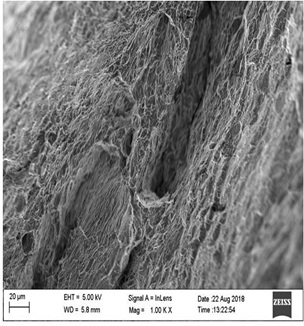
Fig.24. Nugget Zone Material composition at SEM Analysis
At a higher magnification of 150x [7,8], the fine-grained morphology of the fracture surface is visible. Figure 6.6:
This SEM image shows a 250x magnification of Figure 6.3 [34,35]. The damaged surface caused small cracks perpendicular to the stress path. Fractures appear as intergranular cracks extending along the direc-tion of grain movement in the heat affected zone. (See microstructures in Figures 6.6 and 6.7) [9, 10].
A 250x SEM image of the fracture surface is shown in Figure 6.7 [31,32].
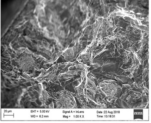
Fig.25. Nugget Zone Material composition at SEM Analysis.
Brittle fracture morphology exhibits fine- grained fractures and no pitting. Figure 6.8 shows a fractured area with large pits [25,29] that may indicate cracks in the material surface. A giant valley formed in the fracture surface was resolved at 500x magnification. Another fractured region [40] with deep valleys present on the fractured material of the sample can be seen in Figs 6 and 9.
Two equivalent magnesium alloys AZ31/AZ31, AZ91/AZ91, similar or dissimilar to AZ31/AZ31, were found to be effectively joined. This technology is also used in military and aerospace structural frames and equip-ment. This his FSW technology reduces overall weight compared to previous aluminum alloys.
This is one of the most cost effective techniques he uses to join two metals during the fusion process. In this procedure, you learned about material stress, strain, elongation, failure, and SEM analysis that helps you understand how materials behave at the micron level. By utilizing this substance, we can support the human body more comprehensively, and future effects are expected.
This technical survey shows four known and limited his MOO benchmark issues.
BNH, DEB (CONSTR), OSY, SRN, TNK. Some of the problems that MOEA may face are his MOGA-II im-plemented in modeFRONTIER and his NSGA-II, and the author's cNSGA-II implemented in his MATLAB. One elite was investigated using his algorithm. At the same time, his two constraint handling techniques, the penalty function approach and the constrained tournament method, were also considered. MOGA-II uses the first method, NSGA-II and cNSGA-II use his second method.
Articulos:
[1] M.M. Avedesian, H. Baker, ASM Specialty Handbook, Magnesium and Magnesium Alloys, ASM International, USA, 1999.
[2] M. Yugandhar,B. Prabhakar Kammar, S. Nallusamy, "Experimental Study and Analysis of Friction Stir Welding on Az-91Mg Alloy by using SEM,"International Journal of Engineering Trends and Technology, vol. 70,no.10,pp.111to123,2022.Crossref, https://doi.org/10.1444 5/22315381/IJETT-V70I10P213.
[3] M. Yugandhar, B. Prabhakar Kammar, S. Nallusamy, "Experimental Investigation on Similar and Dissimilar Materials of AZ31/AZ91 Mg Alloys by Friction Stir Welding," International Journal of Engineering Trends and Technology, vol. 70, no. 11, pp. 338-352, 2022. Crossref, https://doi.org/10.14445/22315381/IJETT- V70I11P236.
[4] F. Czerwinski, F. Czerwinski (Ed.), Welding and Joining of Magnesium Alloys, Magnesium Alloys – Design, Processing and Properties, InTech,Croatia, 2011. ISBN: 978-953-307-520-4.
[5] R.S. Mishra, Z.Y. Ma, Mater. Sci. Eng. R Rep. 50 (2005) 1–78.
[6] R.S. Mishra, P.S. De, N. Kumar, Friction Stir Welding and Processing:Science and Engineering, Springer International Publishing, Switzerland, 2014, doi:10.1007/978-3-319-07043-8_2.
[7] A.C. Somasekharan, L.E. Murr, Mater. Charact. 52 (204) (2004) 49–64.
[8] C.Y. Lee, W.B. Lee, Y.M. Yeon, S.B. Jung, Mater. Sci. Forum 486– 487 (2005) 249–252.
[9] ASTM Standard, E8/E8M-11. Standard Test Methods for Tension Testing of Metallic Materials, ASTM International, West Conshohocken, PA, USA, 2009, doi:10.1520/E0008_E0008M-11.[
[10] R.W. Messler Jr., Principles of Welding: Processes, Physics, Chemistry and Metallurgy, Wiley India Pvt. Ltd, New Delhi, 2004.
[11] R.S. Parmar, Welding Engineering and Technology, Khanna Publishers,New Delhi, 2010.
[12] Joining of AZ31 and AZ91 Mg alloys by friction stir welding B. Ratna Sunil a,*, G. Pradeep Kumar Reddy b, A.S.N. Mounika a, P. Navya Sree a,P. Rama Pinneswari a, I. Ambica a, R. Ajay Babu a, P. Amarnadh a, Journal of Magnesium and Alloys 3 (2015) 330–334.
[13]. Prakash kumar sahu, Sukhomay pal (2015) Multi response optimization of process parameters in friction stir welded AM20 Mg alloy by taguchi grey relational analysis, Journal of Mg and alloys 3 36- 46.
[14]. V.Jaiganseh,P.Sevvel (2015), Effect of process parameters on Microstructural characteristics and mechanical properties of AZ80A Mg alloy during Friction stir welding, The Indian Institute of Metals 68:S99-S104.
[15]. Bhukya Srinivasa Naik et.al.(2015),Residual stresses and tensile properties of Friction stir welded AZ31B- H24 Mg alloyin lap configuration, The Minerals, Metals and Materials society.
[16]. S.Mironov et.al.(2015),Microstructure evolution during Friction stir welding of AZ31 Mg alloy,ActaMaterialia301-312
[17]. Sevvel P, Jaiganesh V (2014), Characterization of mechanical properties and microstructural analysis of Friction stir welded AZ31B Mg alloy through optimized process parameters, Procedia Engineering 97: 741-751.
[18]. B.S.Naik, D.L.Chen et.al (2014), Texture development in a Friction stir lap welded AZ1B Mg alloy, The Minerals, Metalsand Materials society.
[19]. Yong zhao et.al.(2014),Microstructure and mechanical properties of Friction stir welded MG2Nd- 0.3Zn- 0.4Zr Mgalloy,ASMinternational JMEPEG 23:4136-4142.
[20]. S.Ugender, A.Kumar et.al (2014), Microstructure and mechanical properties of AZ31B Mg alloy by Frictionstir welding, Procedia materialscience 6:1600-1609.
[21]. Inderjeet Singh, Gurmeet Singh Cheema et al.(2014),An experimental approach to study the effect of welding parameters on similar friction stir welded joints of AZ31B-O Mg Advances in Materials Science and Engineering: An International Journal (MSEJ), Vol. 2, No. 4, December 2015 17 alloy,Procedia engineering 97:837-846.
[22]. S.Rajakumar, A.Razalrose (2013),Friction stir welding of AZ61A Mg alloy, Advanced manufacturing technology68: 277-292. 11. S.H.Chowdhury et al.(2012),Friction stir welded AZ31 Mg alloy, microstructure, texture and tensile properties, The minerals, metalsand materialssociety.
[23]. A.Razal rose, K.Manisekar et.al.(2011),Influences of welding speed on tensile properties of Friction stir welded AZ61A Mgalloy.JMEPEG 21:257-265. 13. K.L.Harikrishna Et.al.(2010),Friction stir welding of Mg alloy ZM21,Transactions of the indian institute of metalsvol 63.807-811.
[24]. G.Padmanabhan, V.Balasubramanian (2009) ,An experimental investigation on friction stir welding of AZ31BMgalloy. Journalofadvanced manufacturingtechnology49:111-121.
[25]. R.S.Pishevar et.al. (2015) Influences of friction stir welding parameters on microstructural and mechanical properties of AA5456 (AlMg5) at different lap joint thicknesses.JMEPEG DOI: 10.1007/S11665-015-1683.
[26]. A.Kouadri-henni et.al.( 2014) Mechanical properties, microstructure and crystallographic texture of Magnesium AZ91-D alloy welded by friction stir welding. Metallurgical and materials transactions vol 45A.
[27]. Sevvel .P et.al. (2014) characterization of mechanical properties and microstructural analysis of friction stir welded AZ31B Mg alloy through optimized process parameters.procedia engineering 97:741- 751.
[28]. J.Yang, D.R.Ni et.al.(2013) Strain controlled low cycle fatigue behavior of friction stir welded AZ31 Magnesiumalloy. Metallurgicalandmaterialstransactionsvol 45A.
[29]. J.Yang et.al.(2012) Effects of rotation rates on microstructure, mechanical properties and fracture behavior of friction stir welded AZ31 Magnesium alloy. Metallurgical and materials transactions vol 44A.
[30]. Lechoslaw Tuz et.al. (2011) Friction stir welding of AZ-91 and AM lite magnesium alloys.Welding international ISSN:0950-7116. [31]. Kazuhiro Nakata (2009) Friction stir welding of magnesium alloys. Welding international ISSN: 0950- 7116.
[32]. B.Ratna sunil et.al.(2015)Joining of AZ31 and AZ91 Mg alloys by friction stir welding. Journal of magnesiumand alloys.
[33]. Juan chen et.al.(2015)Double sided friction stir welding of magnesium alloy with concaveconvex tools for texture control. Materials and design, Elsevier publications vol 76.
[34]. H.M.Rao et.al.(2015)Friction stir spot welding of rare earth containing ZEK 100 magnesium alloy Materialsand design, Elsevierpublications vol 56.
[35]. A.Dorbane et.al.(2015)Mechanical. Microstructural and fracture properties of dissimilar welds produced by friction stir welding of AZ31B and Al6061.material science and engineering: A Elsevier publications.
[36]. R.Z.Xu et.al.(2015) Pinless friction stir spot welding of Mg-3Al- 1Zn alloy with interlayer journal of material science and technology elsevier publications.
[37].S.Malopheyev et.al.(2015) Friction stir welding of ultra fine grained sheets of Al-Mg-Sc-Zr alloy ,Materials science and engineering A: vol 624 : 132-139. Elsevier publications.
[38]. H.M.Rao et.al.(2015) Effect of process parameters on microstructure and mechanical behaviors of friction stir linear welded Aluminium to Magnesium, Material science and engineering :A vol 651:27- 36.elsevier publications.
[39]. Banglong Fu et.al.(2015)Friction stir welding process of dissimilar metals of 6061- T6 aluminium alloy to AZ31B Mg alloy.Jurnal of material processing technology vol 218:38- 47,elsevier publications.
[40]. Mohammadi et.al.(2015) Friction stir welding joint of dissimilar materials between AZ31B magnesium and 6061 aluminium alloys: microstructure studies and mechanical charectarizations,material characterization vol 101:189-207,elsevierpublications.

Mr.M.Yugandhar * 1 Mechanical Engineering Department, 1Research Scholar, ( New Horizon College of Engineering_Banglore).India-560103. e-mail: yugandhar077@gmail.com Phone: +91 6301012889.